


Example of a Pivot Table
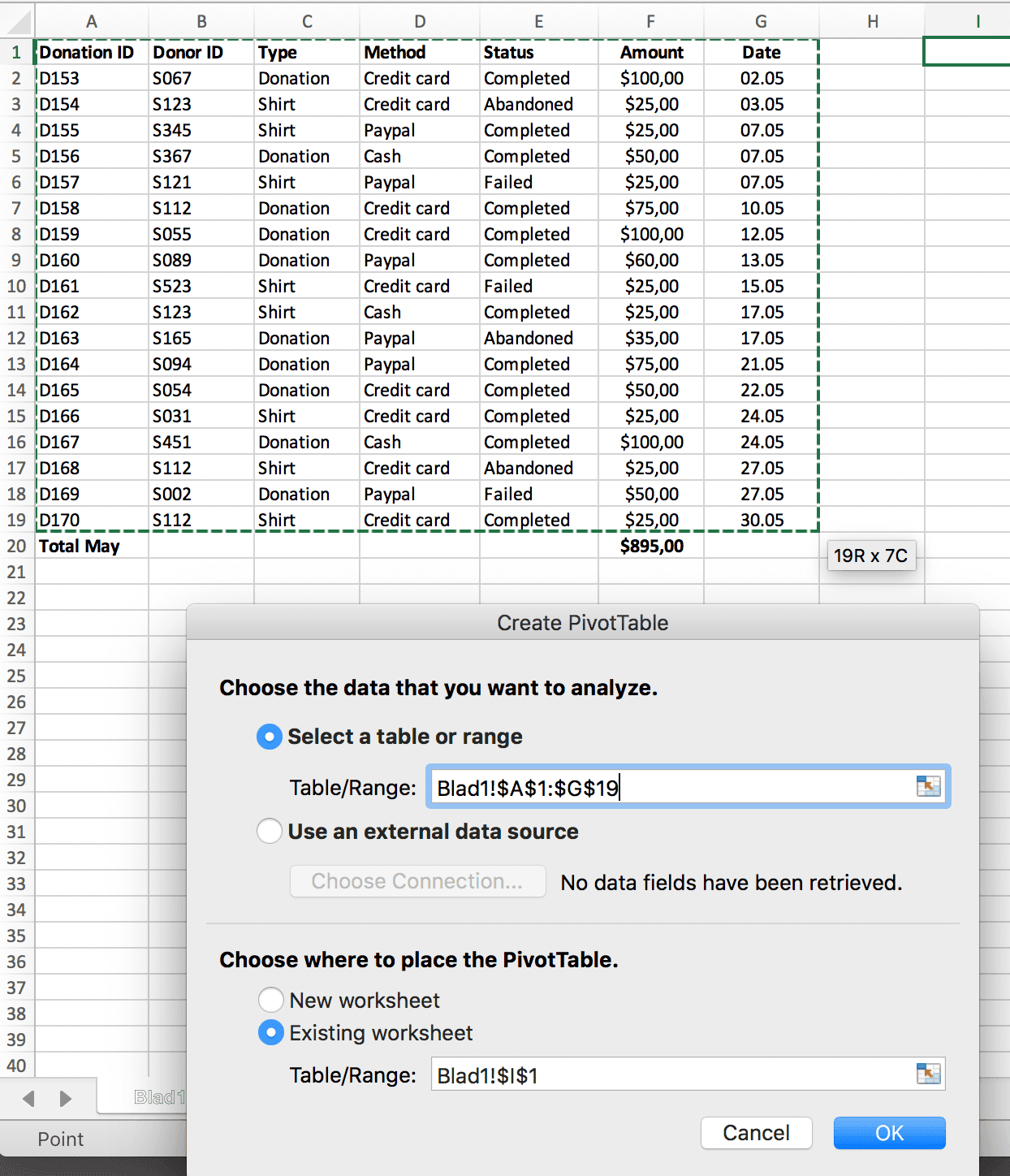
Below you’ll find a table with donations made to a charity organization in May. Each donation has an ID and a donor. Each donor also had a unique ID. Donors can donate in two ways: they can donate money without anything in return, or they can buy a t-shirt. The payment can be made by credit card, Paypal or cash and can reach three different statuses: completed, failed and abandoned. Last, but not least, every donation has a value in Dollars ($).

In the table above we see a total amount of donations of $895. This total amount however is a sum of all donations, including the ones that were abandoned and the ones that failed. The amount that will be transferred to the bank account will only equal the sum of transactions with status ‘Completed’. To find this sum, we’ll use a pivot table.
Step 1 – Insert a Pivot Table
Under ‘Insert’ in the navigation bar, choose ‘PivotTable’.
Step 2 – Select a range
A popup appears titled ‘Create PivotTable’. Select a cell range or table in your workbook that contains the source data. In our example below you see the result of our selection Table/Range: Blad1!$A$1:$G$19. Press ‘OK’ when you’re done.
Step 3 – Compose your Pivot Table
Next you can assemble your PivotTable in the screen ‘PivotTable Fields’. Ask yourself which information you are looking for. In this example we are looking for the total amount of ‘Completed’ donations.

In the ‘PivotTable Fields’ box we select ‘Donation ID’ and we drag-and-drop it to the ‘Rows’ box.

The new table now shows the amount of times each Donation ID appears in the original table. This is, obviously, once per ID.

Next we drag the field name ‘Status’ to the ‘Columns’ box.

The Pivot Table we’ve created now shows per donation whether it was completed, abandoned or failed. We know the sum of donations per status, but we don’t know the sum of amount per status yet. To find the answer we’ll select and drag field name ‘Amount’ to the ‘Values’ box and we’ll remove the current content (Count of Donations ID).
N.B. You can remove content by simply dragging it outside the box (make sure you don’t accidentally drop it inside another box!)

The final composition of our Pivot Table shows us that we’ve received a total amount of $710 of completed donations in May. The other transactions were either abandoned or failed.