Excel HLOOKUP Function: Syntax, Examples & How to Use It

HLOOKUP is a powerful Excel function that helps you search for a specific value across a row (called the ‘table array’) and retrieve data from another row in the same column. Whether you’re working with dates, sales data, or other key information, HLOOKUP allows you to quickly find and return values horizontally. HLOOKUP stands for ‘Horizontal Lookup’ and is essential for anyone looking to streamline data searches in Excel.

HLOOKUP Example

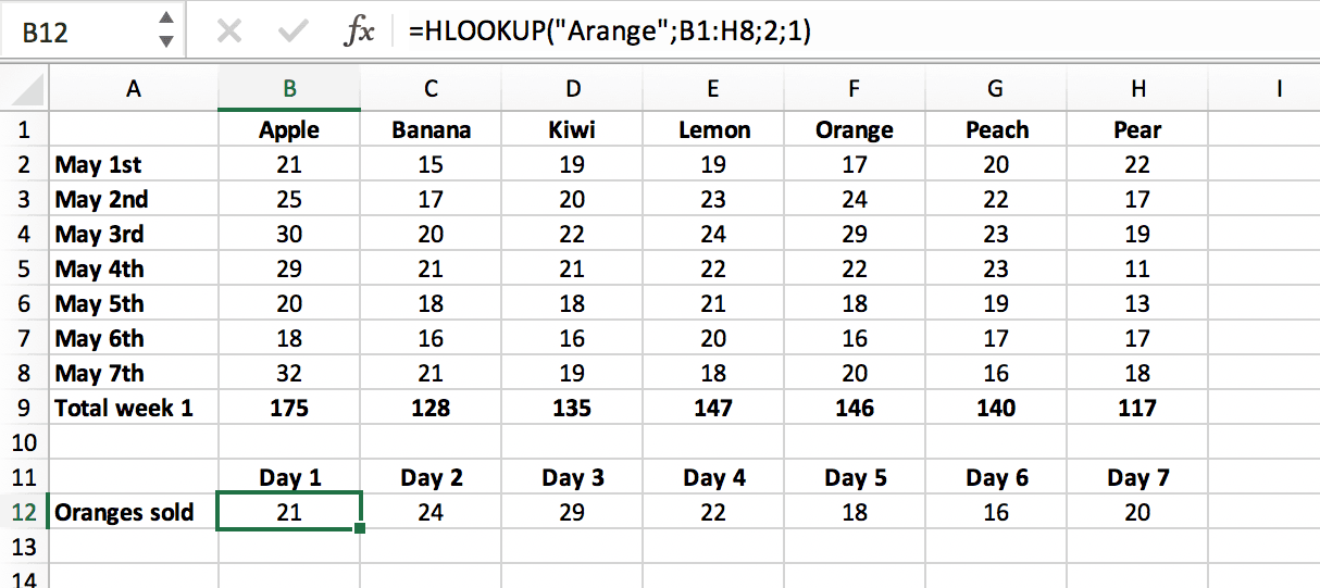
In our example we show how many pieces of fruits are sold per day in the first week of May. We want to find out how many oranges were sold each day of the week.

First, select the cell in which you want to publish the amount of oranges that was sold on the first day.

In the selected cell we type:

=HLOOKUP(

Next, we select the value from row 1 that we want to look up—in this case, ‘Orange’ in cell F1. We can enter this lookup value either as a string ("Orange") (image 1) or as a cell reference (F1) (image 2).

Image 1, Excel HLOOKUP example: Using the string ‘Orange’ as the lookup value

Image 2, Excel HLOOKUP example: Using cell reference ‘F1’ as the lookup value

Next, we enter ; and select the table array where we want to look up the value and retrieve the result. In this case, the selected range is B1:H8.

Next, we enter a semicolon (;), followed by the row number within the selected range where we want to retrieve the value. In this case, it’s row 2 (for Day 1). After that, enter a semicolon (;) and 0 or FALSE to specify that we want an exact match for the lookup value ‘Orange’.

After pressing Enter, the HLOOKUP formula returns the number of oranges sold on Day 1. While this example is simple, HLOOKUP becomes incredibly useful in more extensive spreadsheets, where it can quickly retrieve data from large tables based on different criteria.

To find the sales data for Day 2, simply copy the HLOOKUP formula and update the row number from 2 to 3, like this:

=HLOOKUP("Orange", B1:H8, 3, FALSE).

You can repeat this process for each formula within the range B12:H12. While this example uses a small list of dates, imagine working with a much larger dataset spanning several years. In such cases, HLOOKUP (and VLOOKUP) allows you to change a value in one worksheet, and it will automatically update in all other relevant places.

But what if you’re not sure about your lookup value? In that case, you can use an approximate match by changing the last argument from FALSE to TRUE.

Approximate match

In this example, we enter the word ‘Ornage’ into the HLOOKUP function, as we’re unsure about the spelling of the value we’re looking for. Because the formula is designed to find an exact match, it can’t find ‘Ornage’ in the table array and returns the standard Excel error #N/A.

Now, let’s modify the HLOOKUP function by changing the final argument from 0 (or FALSE) to 1 (or TRUE):

=HLOOKUP("Ornage", B1:H8, 2, TRUE)

With this change, we’ve told the function to look for an approximate match instead of an exact match. If it can’t find an exact match for ‘Ornage’, it will return the closest match that is less than ‘Ornage’, which in this case is ‘Orange’.

If we enter ‘Arange’ instead of ‘Orange’, the HLOOKUP function will return 21. This is because ‘Arange’ does not match any value in the table exactly, so the function finds the closest match that is less than ‘Arange’—which, based on alphabetical order, is ‘Apple’.